We are experiencing the chaos of the information age, and its technological advents with voracious evolution and expansion. And in the midst of all this we have the advent of Big Data that has reached the delights of many with Data Science, Machine Learning and Artificial Intelligence.
As a result, the idea of mathematical and statistical “models” became the rage, gaining visibility. And among these models we have the most trivial of all: regression.
Have you ever stopped to think about where this term comes from, and what it means in practice? Exactly what you thought: “That’s the basics!” That’s why this series of stories was called “trivialities”, as they are trivialities that sometimes need to be known.
On my journey as a Quant backpacker (which is not that long, but long enough to make these observations) I realized that very simple points or concepts are not known to the overwhelming majority, and that is why I observed a lot of misapplication or erroneous judgment in statistical metrics , and I decided to start writing about it.
As I have academic roots, I brought the questions that will direct this text:
What is regression?
What does this term mean?
Where and when did it appear?
How to apply?
Am I applying it correctly?
And as usual, I’ll start from the beginning (😄😄😄).
The beginnings of the Regression
When we think of this term, the idea of linear statistical regression immediately comes to mind. And yes, that’s right, the term is the same, but why regression? When I think about the meaning of the word, and obviously I already looked it up in a dictionary on the internet, which is the same as going back, regression comes from regressing, returning to a state that has already been overcome or that has evolved but returned to its previous levels. previous ones. It’s like climbing a ladder but going down backwards.
And that’s right (😄), regression is twisting, returning to the previous state. This term was coined in 1875 by an amateur mathematician named Francis Galton, who in some books says he was a first cousin of the famous Charles Darwin. Galton brought to the public the coining of this term, calling it “regression to the mean”.
Why regression to the mean? Did something that moved end up returning to the mean? Yes that’s right. The concept only makes sense when we connect it with classical statistics, or better, with the central limit theorem.
This theorem is a right arm of probability theory, and builds the statement that when the sample size increases, the sampling distribution gets closer and closer to a normal distribution, and this is fundamental in statistical inference. Translating into simpler language: it’s like saying that when we observe nature, we perceive a natural state or a standard, normal state of things.
An example using Brazil, a country with a tropical climate, it is correct to say that the natural state of the climate is heat, as it is sunny many more days a year than cold or rainy, therefore, on average it is hotter, so the normal of Brazil is to have sunny days, but when it rains we can activate the idea of normality, in which the rain can soon stop and the sun and high temperatures return to the scene.
Regression to the mean is exactly that, even if you have days with rain, the “normal” is that there are more sunny days, so rainy days are deviations between the averages, as the average is sunny days. But the term became known even after Galton published a study in 1885 in which he demonstrated, through regression calculations, that the height of children does not tend to reflect the height of their parents, but rather tends to regress towards the population average.
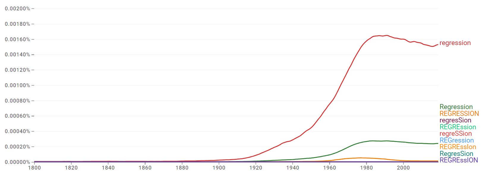
It is possible to see how the term gained scale after use by Galton, using the Google tool: Ngram book viewer.
The use of regression
The application of this method is known to many people, and can be found in different professional areas. But as I come from economic sciences, I will use this line to continue the text.
The economic sciences have econometrics as their quantitative tool, which is the metric for analyzing economic theories. In simpler language, it is the use of classical statistical techniques to analyze and test an economic theory. Economists use a lot of regression in econometrics.
And studying econometrics I learned a lot about the fundamentals of regression analysis. But a few paragraphs above I wrote that regression is returning to your previous state, so how would economists use a matrix like that? For the simple fact that the economy works with the assumption of a state of general equilibrium of things.
The economist has a single objective, and amazingly, it is not to save money, it is to allocate scarce resources to meet unlimited needs. But how does he do this? Artificial intelligence!!! (😄😄😄).
Joking apart. The economist uses optimization as his beacon. Allocating scarce resources to satisfy unlimited needs is only possible by optimizing. And what does optimizing have to do with regression? All! Economists’ assumption of a general equilibrium is only possible using optimization, minimizing costs and maximizing profits, and regressing to the mean or returning to a normal state only reinforces or supports the idea of general equilibrium.
So, I will bring a brief example of application, coming from a study material for economists, the book on basic econometrics by Damodar N. Gujarati and Dawn C. Porter, in which we find an application that is well known among economists: the hypothesis of marginal propensity to consume, or MPC.
Keynes stated: The fundamental psychological law […] is that men [women] are disposed, as a rule and on an average, to increase their consumption as their income increases, but not in the same proportion as the increase in income.(Keynes, John Maynard. The general theory of employment, interest and money. New York: Harcourt Brace Jovanovich, 1936. p. 96.).
So to simplify, we will use an econometric model based on a simple linear regression, but first I need to comment that there is a rationale behind a linear regression, which is the central objective of this text, to talk about some basic points that sometimes fall into oblivion .
An econometric model (statistical/mathematical) aims to represent the reality we are interested in investigating. The model must be able to capture the relationships between reality and theory, so that the theory can be tested. However, this representation of reality is not complete, a model alone is not capable of representing or describing reality as a whole, so it needs to be conditioned and sometimes restricted.
Keynes’ hypothesis brings exactly this idea, with the construction of a consumption function, and without many details, his hypothesis of a relationship between consumption and income seems deterministic or an exact relationship. So, as the model cannot have all the information, it uses the most likely or available information and relies on the premise that the other effects are constant or unchanged, not causing direct influence: ceteris paribus.
I wrote a text about how I see the ceteris paribus condition, and how it helps us understand real-life phenomena. So, returning to the example of Keynes’s hypothesis, he uses ceteris paribus in an intuitive and implicit way, leaving no details, but establishing the premises: “to increase your consumption as your income increases”. So we already have the relationship we need to build our model.
In short, Keynes postulated that the population had a tendency to increase its consumption when its income increases, which was labeled marginal propensity to consume (PMC), and it would be analyzed quantitatively as a rate of variation in consumption, and that this variation would be given in units (say, one dollar) of income, and that it will always be greater than zero, but less than 1, as his observations showed that additional consumption did not have the same level as additional income, that is, people did not they consumed everything they earned and that is why it has to be less than 1.
Specifying the hypothesis-based econometric model
Although Keynes established an apparently positive relationship between income and consumption, he did not stipulate how this relationship happens. To simplify, let’s use “poetic license” and suggest the following functional form for the relationship between income and consumption established by Keynes:
\[ Y = \alpha + \beta X \;\;\;\;\;\;\;\; 0 < \beta < 1 \]
where \(Y\) represents consumption expenditure and \(X\) represents income, and \(\alpha\) and \(\beta\) are the model parameters. These parameters represent the effects generated through the relationship between \(X\) and \(Y\). Sometimes known as marginal effects.
The parameter \(\alpha\) is known as “intecept”, or average value. Generally it demonstrates that where the relationship between the variables between \(X\) and \(Y\) begins. It is the average value, if the marginal effect is null (zero). It’s like saying that, if \(X\) has no influence on \(Y\), then when \(X\) and \(Y\) are related, it is \(\alpha\) that shows the level of this relationship.
The parameter \(\beta\) is known as “angle” or “angular coefficient”, also called the slope of a straight line, it determines the slope of a straight line. A straight line because the relationship between \(X\) and \(Y\) is direct (linear). The angular coefficient is a number that is related to the angle formed between the straight line and the horizontal, describing the slope of the straight line. And when we connect the terms “slope” and “angle”, we can remember the concept of derivation, and that is exactly it, it is the effect of the derivation in relation to \(X\). And we know that in economics the concept of marginality is directly correlated to the concept of derivation, which is why the angular coefficient is known as marginal effect.
And the angular coefficient (\(\beta\)) will be our indicator of the relationship between income and consumption, which we will call Marginal Propensity to Consume. This is already constructed by Keynes’ theory, but we are here trying to work on an idea.
As I mentioned in the paragraphs above, this relationship does not represent a pure and exact reality. Of course, there are many variables that can affect consumption in addition to income, and therefore the model needs an additional specification, which for me is the charm of the linear regression model.To take into account the influences of other variables that were not imposed in this model:
\[ Y = \alpha + \beta X + u \]
where \(u\) is known as the disturbance, or error term of the model. It is a random (stochastic) variable that has probabilistic properties. The error term \(u\) is intended to represent all other factors that affect consumption but are not explicitly imposed here.
The error term is essentially the ceteris paribus condition. It contains all the other effects that interact with Consumption, but they are being nullified, or kept constant/unchanged, that is, there is no variation, so no effect can be felt.
That is, by isolating the effect of income on consumption, we artificially create a kind of general equilibrium, showing that the relationship between \(X\) and \(Y\) is balanced (normal), and that other factors have no influence.
Estimating the model
With data from Table I.1 of the Gujarati basic econometrics book, which refers to the United States economy in the period 1960-2005. Table I.1 uses aggregate consumption to represent model consumption, and GDP to represent income, and thus we will estimate the marginal propensity to consume. With the data in hand, it’s time to go to RStudio and start “the work”. Let’s Code!
Now that we have an output from the experimental model, we can obtain numerical estimates of the parameters that will provide us with an empirical resolution for the consumption function proposed here in this example.
Now that we have an output from the experimental model, we can obtain numerical estimates of the parameters that will provide us with an empirical resolution for the consumption function proposed here in this example.
We can note that the statistical technique of regression analysis is the main tool for obtaining such estimates. After running the model, we obtain the following estimates:
\(\hat{\alpha}\) = -299.6
\(\hat{\beta}\) = 0.7218
Now we can empirically translate the estimated consumption function as:
\[ \hat{Y_t} = \hat{\alpha} + \hat{\beta} X_t \]
\[ \hat{Y_t} = -299,5913 + 0,7218 X_t \]
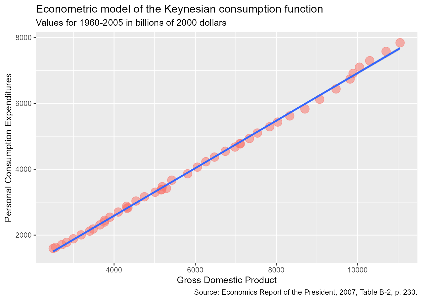
The caret above the Y and the parameters \(\alpha\) and \(\beta\) indicates that this is an estimate. The following graph shows this estimated consumption function (i.e., the regression line).
Show the code
# load librarieslibrary(tidyverse)# building a plot with ggplot2 based on grammar of graphics:tbl_pmc %>%ggplot(aes(x = gdp_x, y = pce_y )) +geom_point(aes(color ="red", size = .7, alpha = .8 )) +geom_smooth(method ="lm", se =TRUE, inherit.aes =TRUE ) +theme(legend.position ="none") +labs(title ="Econometric model of the Keynesian consumption function",subtitle ="Values for 1960-2005 in billions of 2000 dollars",x ="Gross Domestic Product",y ="Personal Consumption Expenditures",caption ="Source: Economics Report of the President, 2007, Table B-2, p, 230.")
The red dots represent our income data (GDP), and the blue line represents the regression line.
As we can see in the model graph, it is possible to say that the regression line (blue) fits the data well, this means that the points (red) on the graph that represent the data are very close to the regression line.
The table of model results and the graph show us that, in this analyzed period (1960-2005), a marginal effect of income (GDP) on consumption behavior of almost 0.72 is estimated.
As I already mentioned, this marginal effect estimate comes from the angular coefficient, which we will now call “Coefficient of the Marginal Propensity to Consume”, and this coefficient is telling us that, in the sampled period, whenever there is an increase of one dollar in income In real terms, on average, there is an additional increase of around 72 cents in real consumption expenditure, that is: for every 1 dollar more, there is, on average, a marginal effect of 72 cents. If it increases by 1 dollar, consumption increases by 72 cents, and the opposite is also true.
Average Marginal Effects
Attention to a critical point: we use the term “average” or we always use the phrase “on average” because the relationship between consumption and income is inexact, that is, it is not a direct causal relationship; and this is very clear in the model graph, as not all red points in the data are exactly on the regression line.
In general terms, we can say that, “[…]according to our data, average consumer spending increases by about 70 cents for every dollar increase in income.
And this reinforces the idea of normality and average. We use the average as the optimal moment, because under normal conditions of temperature and pressure the effect is recognized in the average, because no matter the changes or oscillations, if we believe in the normality that after these variations everything returns to normal, then the average is the central point, that is, the normal.
As I tried to explain before, what we call marginal effects are partial derivatives of the regression equation in relation to each variable in the model; So therefore, the average marginal effects are simply the average of these partial derivatives. In ordinary least squares regression, the estimated slope coefficients (angular and/or \(\hat \beta\)) are marginal effects.
Now we know that on the surface, Keynes’ assumption appears to make sense. We found this positive relationship between income and consumption. However, we still cannot simply accept this value as a confirmation of the Keynesian consumption hypothesis, as it is not enough to just find the effect, it is necessary to test it, and that is science. And following the scientific standard, let’s create a problem question: “Is this estimate sufficiently below unity?” This is to convince us that it is not a result due to chance or a peculiar insight that the data we use is showing.
Testing a hypothesis
Based on the idea of a scientific test, in which the statistical framework is used as a tool, is the marginal effect of 0.72 statistically smaller than 1? If this is true, it will be support for the birth of a theory. This practice of testing, or better said, corroborating or refuting existing economic theories or those that are emerging, based on sample evidence, which is basically what we have just done, has a foundation based on statistical theory, in a field of study known as statistical inference (hypothesis testing).
Let’s consider that the adjusted model we have just put together is a reasonably good approximation of reality, and that is one of the objectives of a model, but we need to be critical and criticize our own model, trying to understand if the estimates obtained are in accordance with the expectations of the theory being tested, which in this case is Keynes’ theory of marginal propensity to consume.
Economist Milton Friedman said that a theory or hypothesis that is not verifiable with empirical evidence may not be admissible as part of scientific research. Whereas Keynes expected the marginal propensity to consume to be positive but less than 1. In our model, we estimate a marginal propensity of about 0.72. But before this figure can be accepted as a confirmation of Keynesian consumption theory, we need to statistically test this estimate to convince ourselves that it is not a result due to chance or a peculiarity of the data we use.
Para isso, iremos utilizar do conceito de teste de hipotese. Nesse teste teremos que lidar com dois tipos de erros possíveis de ocorrer:
A hipótese nula é rejeitada embora seja verdadeira (erro tipo I)
A hipótese nula não é rejeitada embora seja falsa (erro tipo II)
Tip with Title
The significance level of the test is the probability to commit a type-I-error we are willing to accept in advance. E.g., using a prespecified significance level of 0.05, we reject the null hypothesis if and only if the p-value is less than 0.05. The significance level is chosen before the test is conducted.
An equivalent procedure is to reject the null hypothesis if the observed test statistic is, in absolute value terms, larger than the critical value of the test statistic. The critical value is determined by the significance level chosen and defines two disjoint sets of values which are called acceptance region and rejection region. The acceptance region contains all values of the test statistic for which the test does not reject while the rejection region contains all the values for which the test does reject.
The p-value is the probability that, in repeated sampling under the same conditions a test statistic is observed that provides just as much evidence against the null hypothesis as the test statistic actually observed.
The actual probability that the test rejects the true null hypothesis is called the size of the test. In an ideal setting, the size does equal the significance level.
The probability that the test correctly rejects a false null hypothesis is called power.